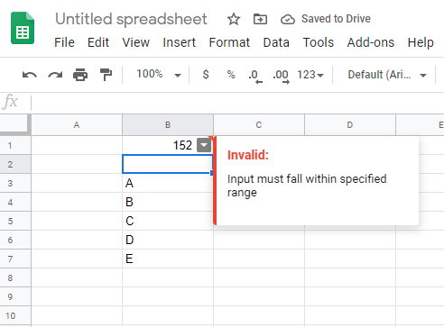
Working with google sheets sometimes requires one to create a dropdown list of items where one can choose from. These items can be numbers, list of items, or even data. The cell where the drop-down appears shows an arrow pointing downwards. In this article, I will give a detailed step by step explanation on how to add a list of items in a cell. The version used to explain makes use of google sheets from windows chrome
Simple steps for adding a dropdown in Google Sheets
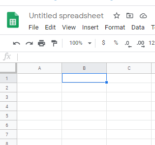
1. Select the cell where you want the dropdown list to appear. In this case, I chose cell B1.
2. Click Data on the upper part of the spreadsheet. A menu appears and here you need to choose data validation as shown below. When data validation is clicked this appears.
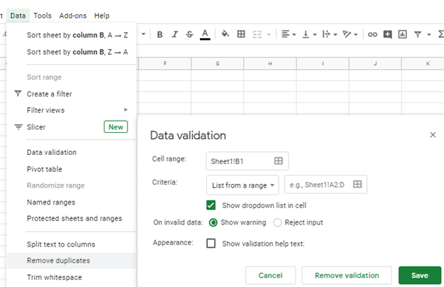
3. Choose the nature of the data you want in the list. In this case, there are several options to make. You can choose a list of items, list from a range, number, text, date, or even checkbox. If you would like to choose from a list that already exists in the google sheet cells you select a list from range option. A list of items can be typed in a space that appears once you click the list of items option.
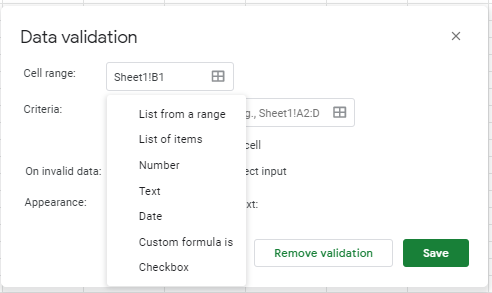
4. In this case, I would like to enter drop-down from a range of values that are in the google sheet cells. Therefore to highlight the options click the icon select data range
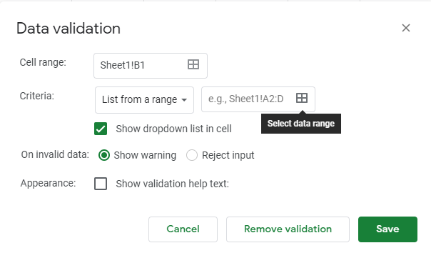
5. Enter the first cell and the last cell where you would like your range to start and end. You can highlight the data that you want to use in the dropdown instead of typing the first and last cells.
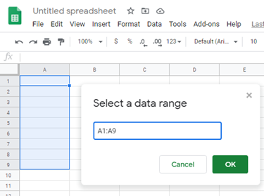
6. Click ok. The dropdown button appears on the cell you chose in the beginning. Once clicked the list of the data items that were chosen appears.
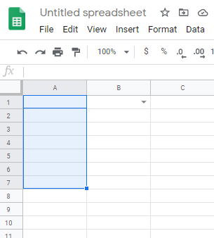
The dropdown list allows people to choose from what appears in the list of values or data items that you entered in the drop-down. Therefore, it will restrict one from making mistakes and errors through the entrance of the wrong data. A warning appears if someone attempts to enter data that differs from what the dropdown requires.
