When using a spreadsheet you interact mainly with rows and columns.
A row in Google sheets is a line of entries going from left to right. It also may refer to a line of objects spaced in an orderly manner example seats in a theatre. Columns, on the other hand, are a vertical line of entries in a table usually read from top to bottom. The use of rows and columns in Google sheets makes your general work presentable and neat. It is also easy to search and retrieve content from the created or existing spreadsheets. Confusions are also limited once the rows and columns are well identified.
The benefit of making rows and columns visible at all points is to keep all data in the spreadsheet clear to all the intended viewers and easier reading.
Step 1
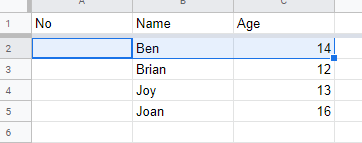
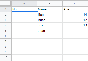
To make the rows or columns visible, first of all, open a blank spreadsheet on Google sheets on your personal computer and insert some general data in it, for our case let us do an example of names and age.
Step 2
After opening and inserting some data in your spreadsheet select the top row which in our case is the one we wish to make it all visible.

Step 3
Having done that, next we navigate to the toolbar, where we have the file, edit, and view, insert, etc. and click on the view button that makes the freeze and other commands visible. Click on freeze.

Step 4
The final step of this procedure will be to select the number of rows to freeze to remain visible. Under freeze command select the number of rows to freeze; in our case, we are just interested in the top row so we select “1 row”.

Having done all those steps you are sure to have made the top row of any Google sheets visible. The top row of your Google sheet will remain visible even when you scroll up and down it will remain highlighted all around as in the case below.
