Keeping the top row visible is one of the quickest ways that you can create the visual reference. This is an important technique because it helps you identify the data that you are sorting even in a long spreadsheet. The cells in the header row will contain information that will describe the information entered in the columns below them. Another thing that I find useful after freezing the top row is changing the color to differentiate it from the rest of the rows.
Apart from freezing rows, you can also freeze the columns using the same method below.
Steps for freezing the first row
1. Open your spreadsheet
2. Customize the row so that it can look unique from other rows. This can be done by either changing the font face, color or weight. Besides, one can change the background color to create a visual contrast to the other cells.
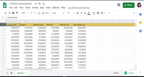
3. Click one cell in the header row
4. Click the View tab located at the top menu to launch another dropdown menu
5. Hover the cursor to freeze rows button in the drop-down menu to launch another sub menu
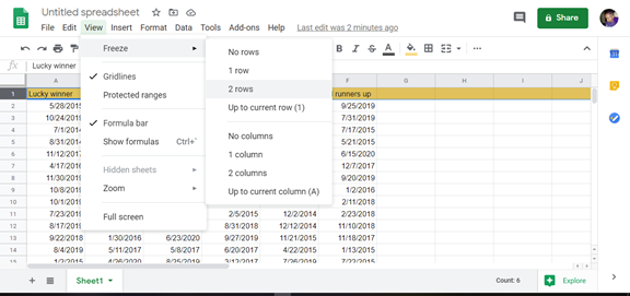
6. To freeze the top header row click “Freeze row 1”
Scroll down to confirm whether your row has been frozen
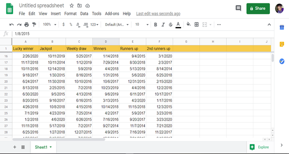
As you can see from the above screenshot our top row is visible even as we scroll further down
More Tips
If you want to keep more than one row visible at once then that is possible too. Google sheets allow you to freeze up to 10 rows and 10 columns. All you need to do is to select the number of rows you want to keep visible in the submenu “Freeze rows”.
Apart from designating a header row, google sheets allow you to designate a header column so that you can navigate easily.
1. Click on any cell in the header column
2. Click the View tab located on the top menu
3. Select freeze columns
4. Click on the number of columns that you want to freeze from the submenu
Hide rows in google sheets
One of the main reason why people want to keep some rows visible it’s to make navigation easy. Another way to improve navigation is hiding some rows or columns
1. Right-click the row header
2. Click hide row button on the menu that will appear
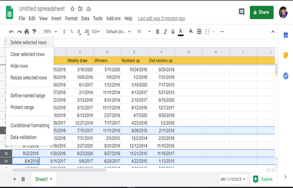
3. The rows selected will disappear but with some arrows appearing on either side to signal hidden rows
4. Click on the arrows to show the hidden rows in google sheets

