Conditional formatting in spreadsheets allows you to apply specific formatting to the cells if they meet a certain condition. Mostly is used to differentiate the data or any information in a spreadsheet to emphasize something in it. You can use conditional formatting to identify duplicate data within a spreadsheet. Google Sheets offers several formats for cells, rows, or columns to change text or background if a given condition is met.
Step 1
On your personal computer, open a spreadsheet in Google Sheets or even open an existing file.
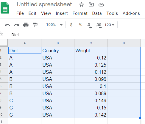
Step 2
In this step, select the cells you wish to apply the conditional formatting rule.
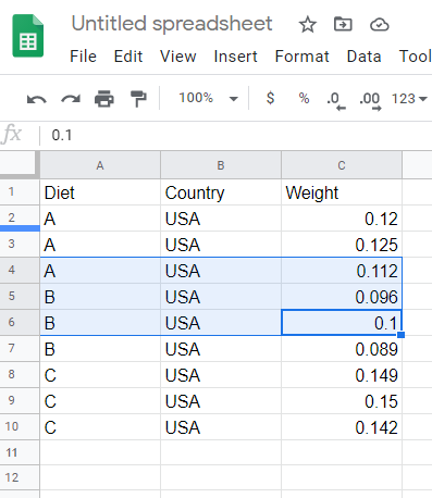
Step 3
After selection, Click format a toolbar will pop out then scroll down and click conditional formatting
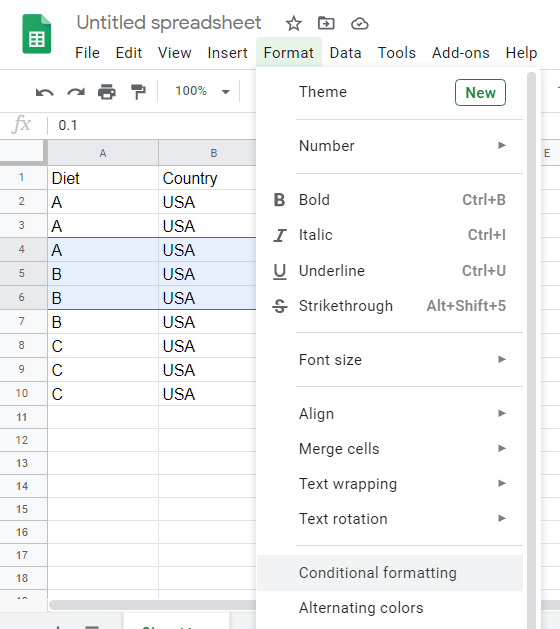
Step 4
In this step, you can create a rule to be applied in your selected cells. For our case, we are going to create a color rule to be applied to the cells. Under the “Format cells if” our option is “single color”.
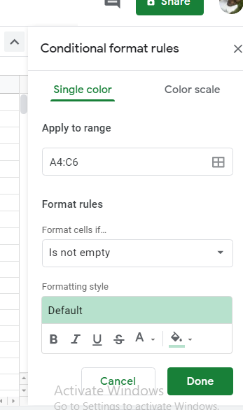
Choose custom color
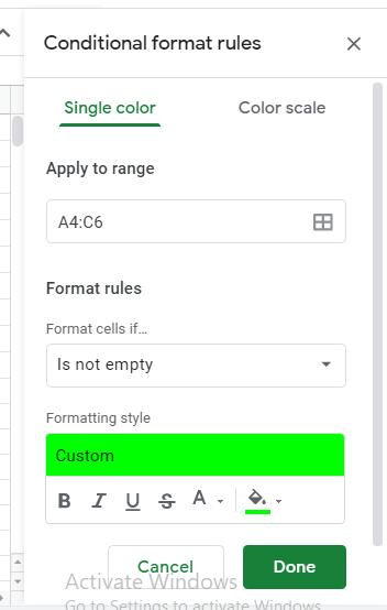
Step 5
Click Done then the rule will be applied.
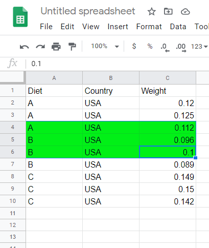
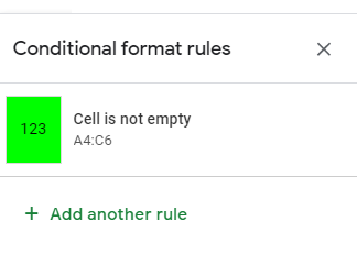
In case you want to remove that rule, click to the rule, and remove it. These rules are in the order list if any rule found to be true in your spreadsheet will automatically define the format of range or the cells. When you try to copy and paste within the cells that already have the formatting rule the rule will be automatically applied.
To remove rule click on the rule or to add rule click the plus sign icon.
You can use conditional formatting rule across an entire row this might be based on the value in a single cell. This highlights rows of data in a table if there is a value that exceeds some threshold.
Conditional formatting can help you be able to understand spreadsheets and create a more readable spreadsheet, it also helps to track goals and giving you a visual indication of your progress.

