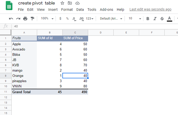
Pivot tables will let you analyze large amounts of data and narrow down large data sets to see the relationships between data points. Pivot table in Google Sheets are used to summarize data, making it easier to understand all the information contained in your spreadsheet
Google sheets allow you to make changes to the file without having to destroy the original document. When you are done making changes, you can simply download it where sheets are going to convert it back to excel files, ready to be used by Microsoft excel once again.
For those who might have been used to Microsoft excel where you only need to select data to be included in the table then click “CTRL+T” for Windows and “Apple +T” for MAC, or the Format as Table option in Excel standard toolbar, must find it challenging to insert Table in Google sheets since there is no direct option for Tables.
Steps for creating a pivot table
1. Open your spreadsheet First; select the data you need to be included in the table.
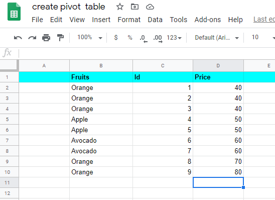
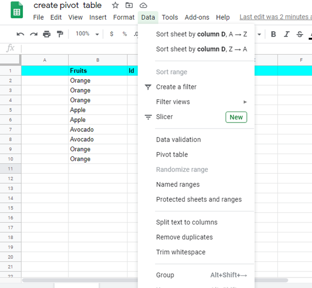
2. In the menu at the top toolbar, click ‘Data’ then select ‘Pivot Table’.
3. Click creates on the pop-up window that appears once you click on the ‘Pivot table’.
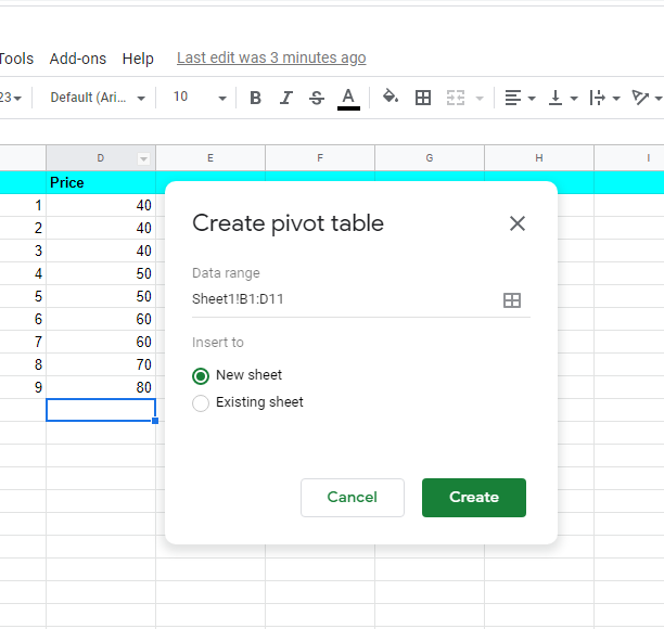
A new sheet opens up at the bottom of the screen as shown.
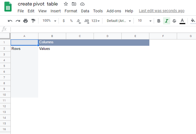
4. Use the Pivot table editor window which pops up at the right side of the screen to edit your table.
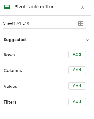
5. Click on rows and select what is to appear on the rows, Click on add Columns then choose what is to appear on the columns. Your table is created as per your editing desires.
