You can easily notice that by default, the cells of every new spreadsheet always have the same size. Once you begin entering or pasting your information into your spreadsheet, it’s easy to customize columns to make it better fit your data. Also in Google Sheets, if you want to link or combine data from multiple cells together, you don’t have to merge them. You can use the CONCAT, CONCATENATE method, and JOIN functions to combine them in one cell. These functions range from the simplistic CONCAT to the complex “JOIN” CONCATENATE it
offers the most flexible way, as it allows you to manipulate the linked data with operators and additional content use the following methods and follow step by step. In addition, every row and column of a new spreadsheet is always set to the same height and width.
Method
CONCAT Function
In our case, we are going to use the CONCAT function to combine our data in the data cells, but it has some limitations. The first limitation is that you can only link two cells and it does not support operators to configure how to display the two linked data.
1. To use CONCAT, open your Google Sheets spreadsheet and click an empty cell within your document. Type =CONCAT (Cell A, Cell B), but make sure you have replaced Cell A and Cell B in your spreadsheet. According to our case, we are using Cell A and C, in our case we are going to include column D for a combination of our cells as shown below,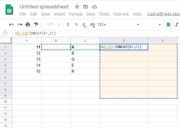
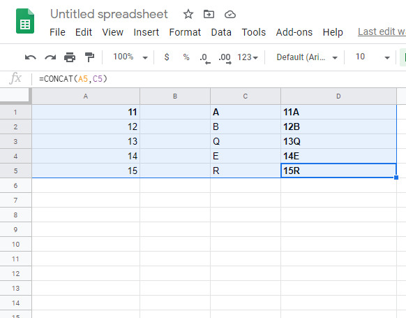
2. Place your cursors to the column you want to combine your cells and make sure you have selected the cell, then press you Enter for every cell, and your combination will be shown as follows or drag your cursor down the column. Use the same to all other cells of the column D. follow step-by-step instructions, make you understand how to enter the same formula into all selected cells at a time as follows,
See the OUTCOME bellow.
.

