Google sheets represent data in different formats such as in graphs or even charts that are created or include the use of axes that are x and y-axis.
An axis can mean an imaginary line about which a body rotates on, a good example is a spherical object that revolves on its axis. It can also mean a fixed reference line for the measurement of coordinates or even a straight central part to which other parts are connected.
There are two major types of axes; x-axis and y-axis. The X-axis is horizontal running from left to right whereas the y-axis is vertical running from top to bottom. The x and y-axis meet at a point called the origin.
The following are steps to make two y-axes in Google sheets;
Step 1
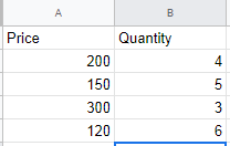
Firstly open a blank spreadsheet on Google sheets on your personal computer, create some data by inserting, for example, a column of price and quantity.

Step 2
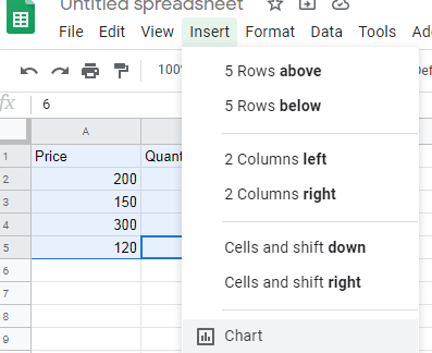
Having created the data, highlight the two columns together with their data, and click on insert to enable you to insert a chart.

Step 3
Once you have prompted the chart command it brings forth a chart of quantity vs. price and on the far right, you can see the chart editor. Under the chart- editor click on the drop-down on the scatter chart to select the type of chart you wish to use, in our case we are going to use a column chart.

Step 4
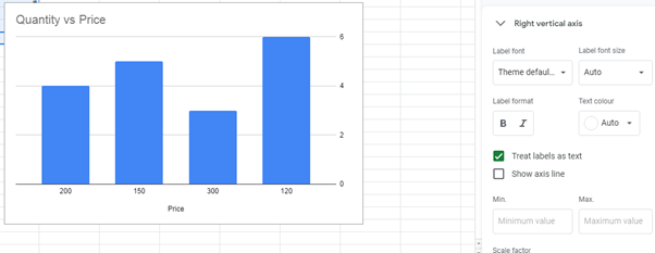
A column chart of quantity vs. price will appear, to make two y-axes we double click on the chart we have just created, it will appear as if highlighted. On the right-hand side select on customize and under that click on series. Change to the right axis under “axis” if it is originally on the left axis.

Step 5
Finally, click on the right vertical axis that appears on the bottom of the chart editor window and make your changes based on your needs.

As in the case of the y-axis, you cannot add a second x-axis.


